Electronic Controls Design E51-0386-40 Super MOLE® Gold 2 User Manual ECD M O L E MAP Users Help System 3 0 6
Electronic Controls Design Inc Super MOLE® Gold 2 ECD M O L E MAP Users Help System 3 0 6
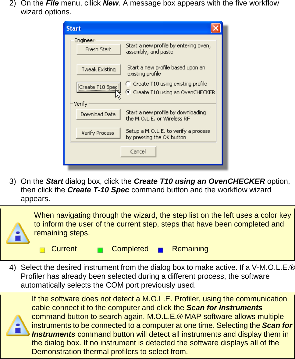
Contents
- 1. User Manual part 1 of 3
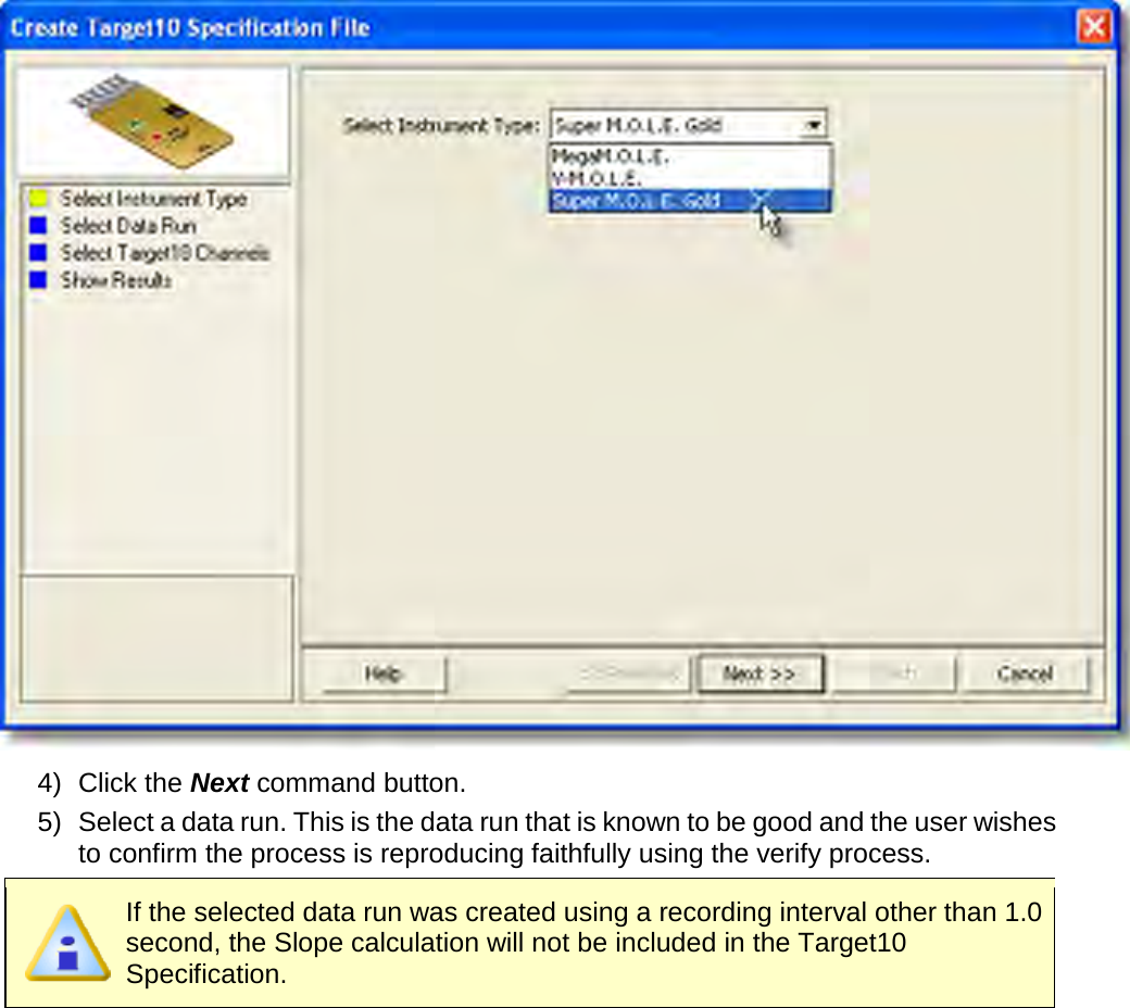
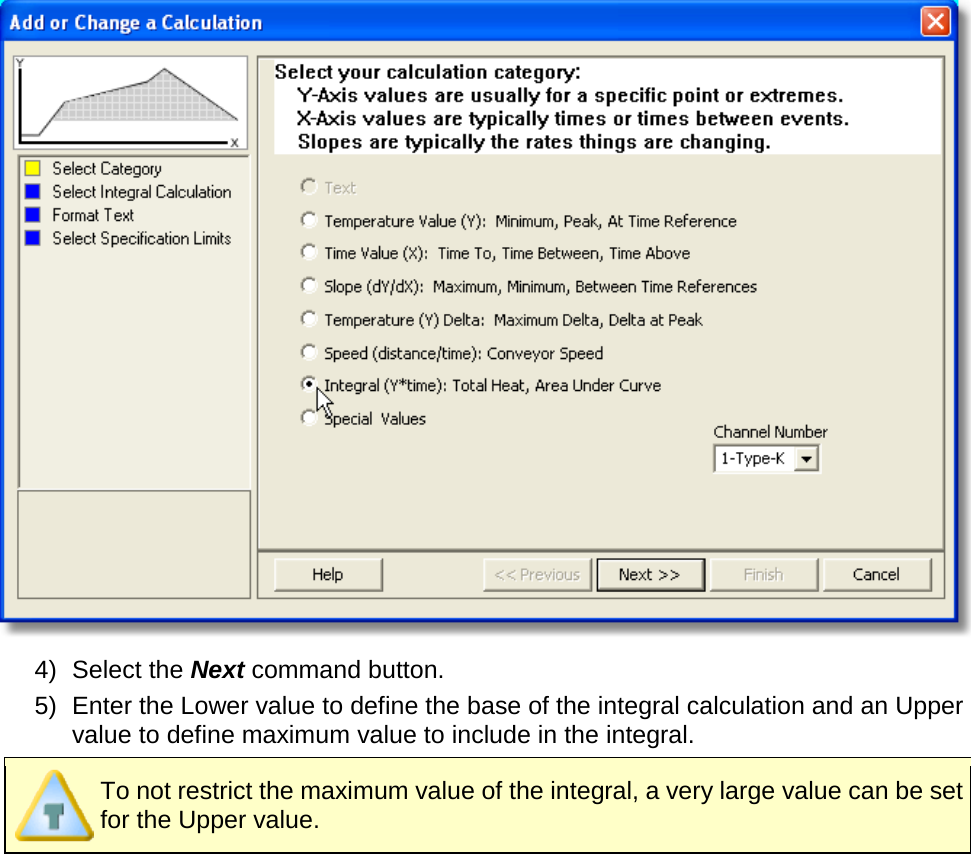
- 2. User Manual part 2 of 3
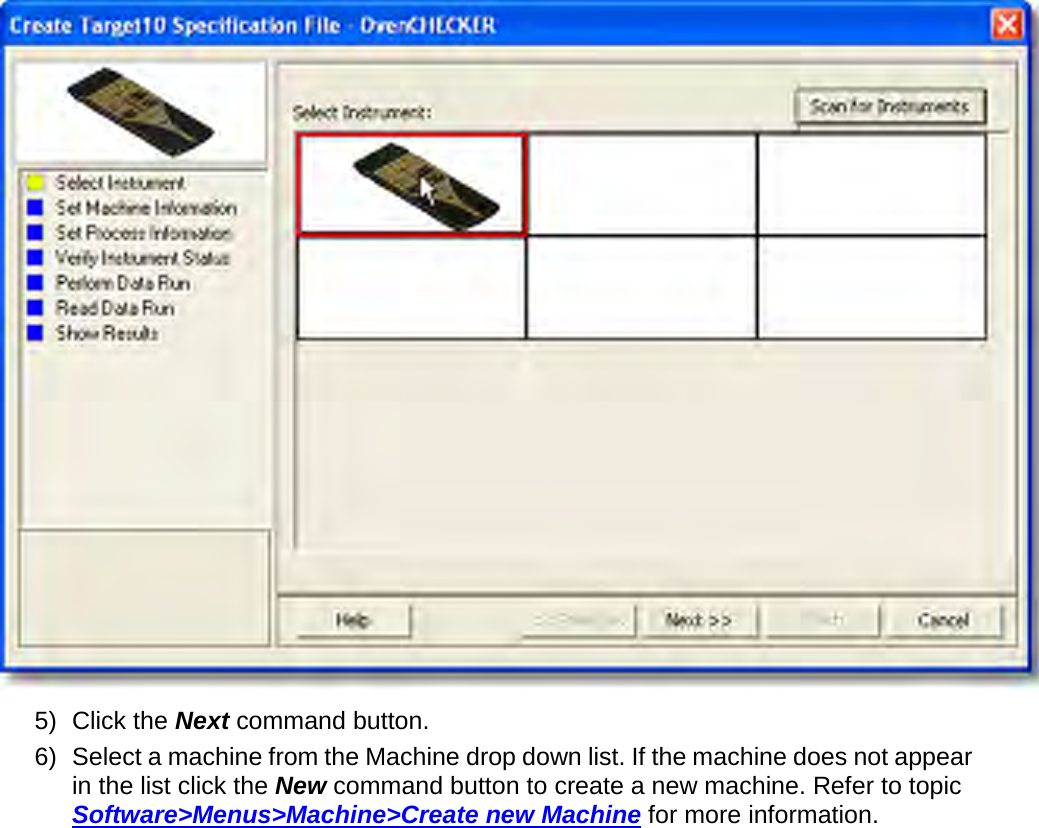
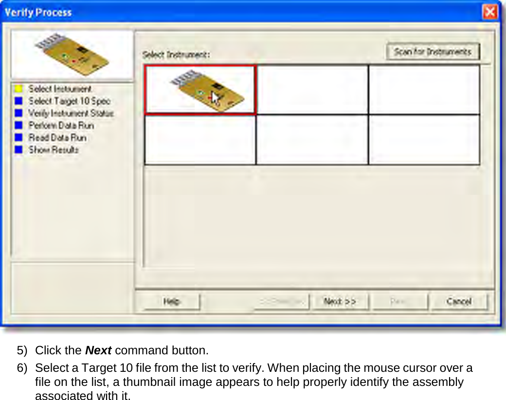
- 3. User Manual part 3 of 3
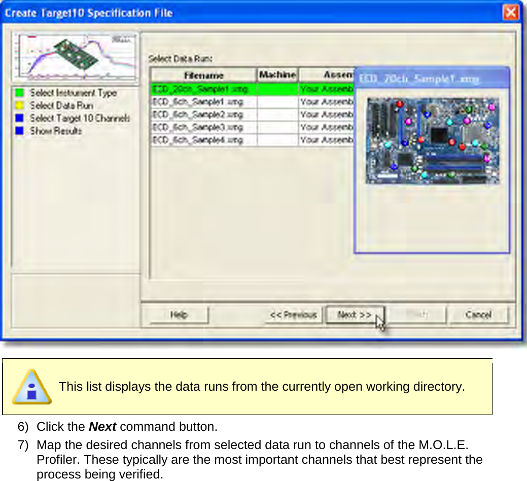
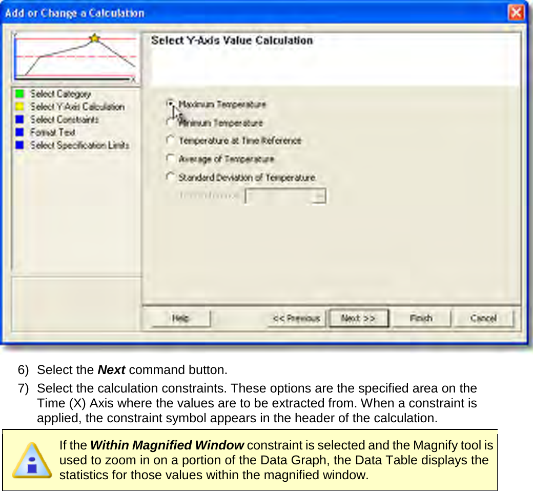
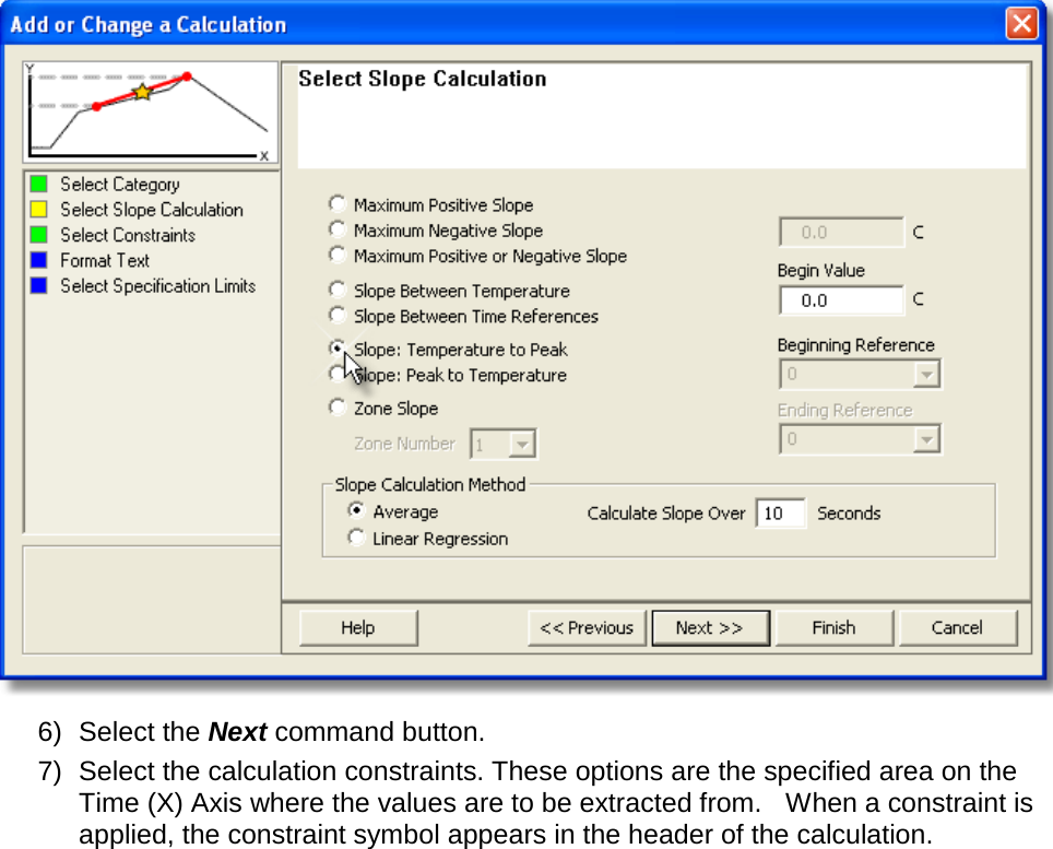
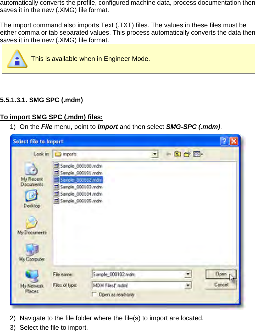
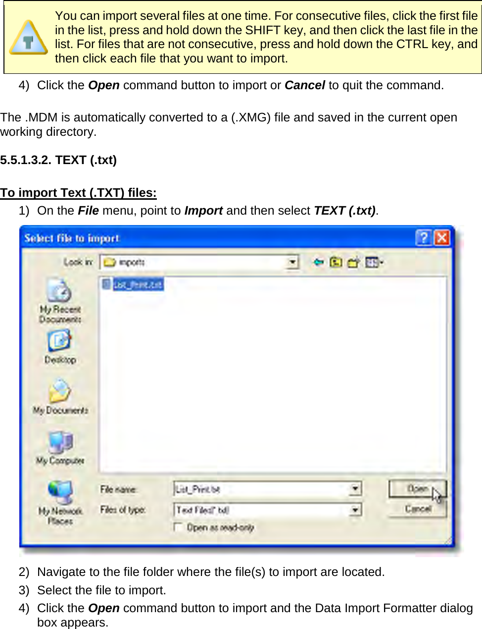
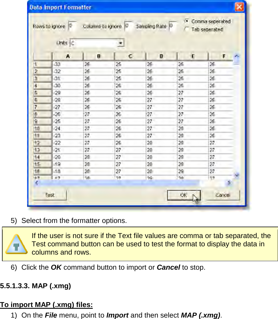
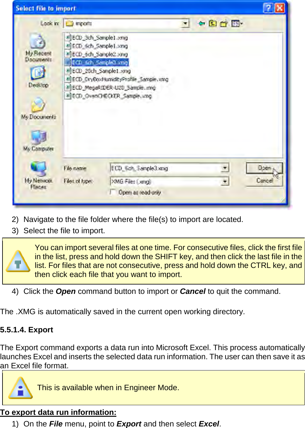
User Manual part 2 of 3
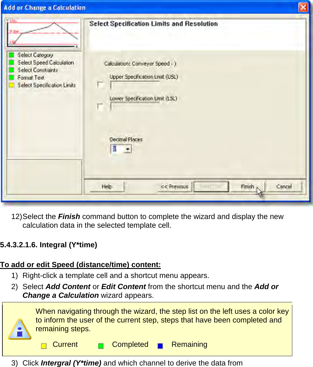

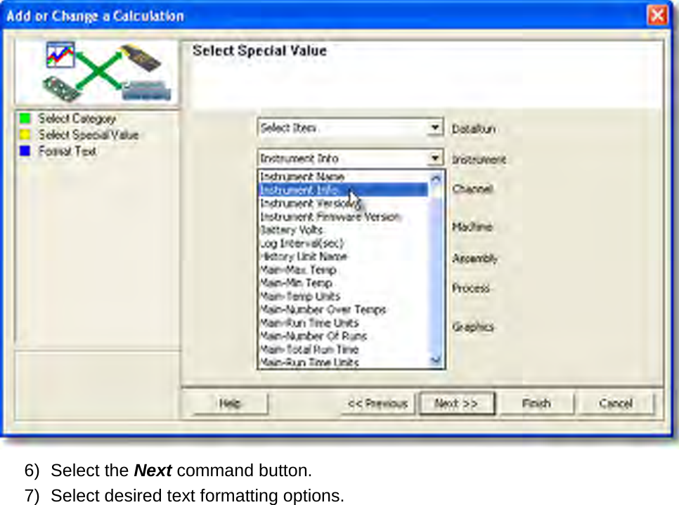

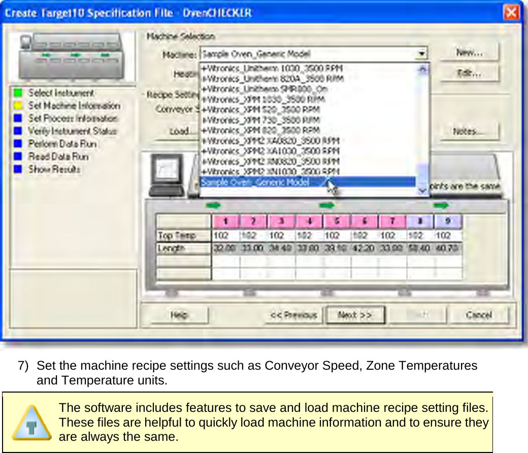
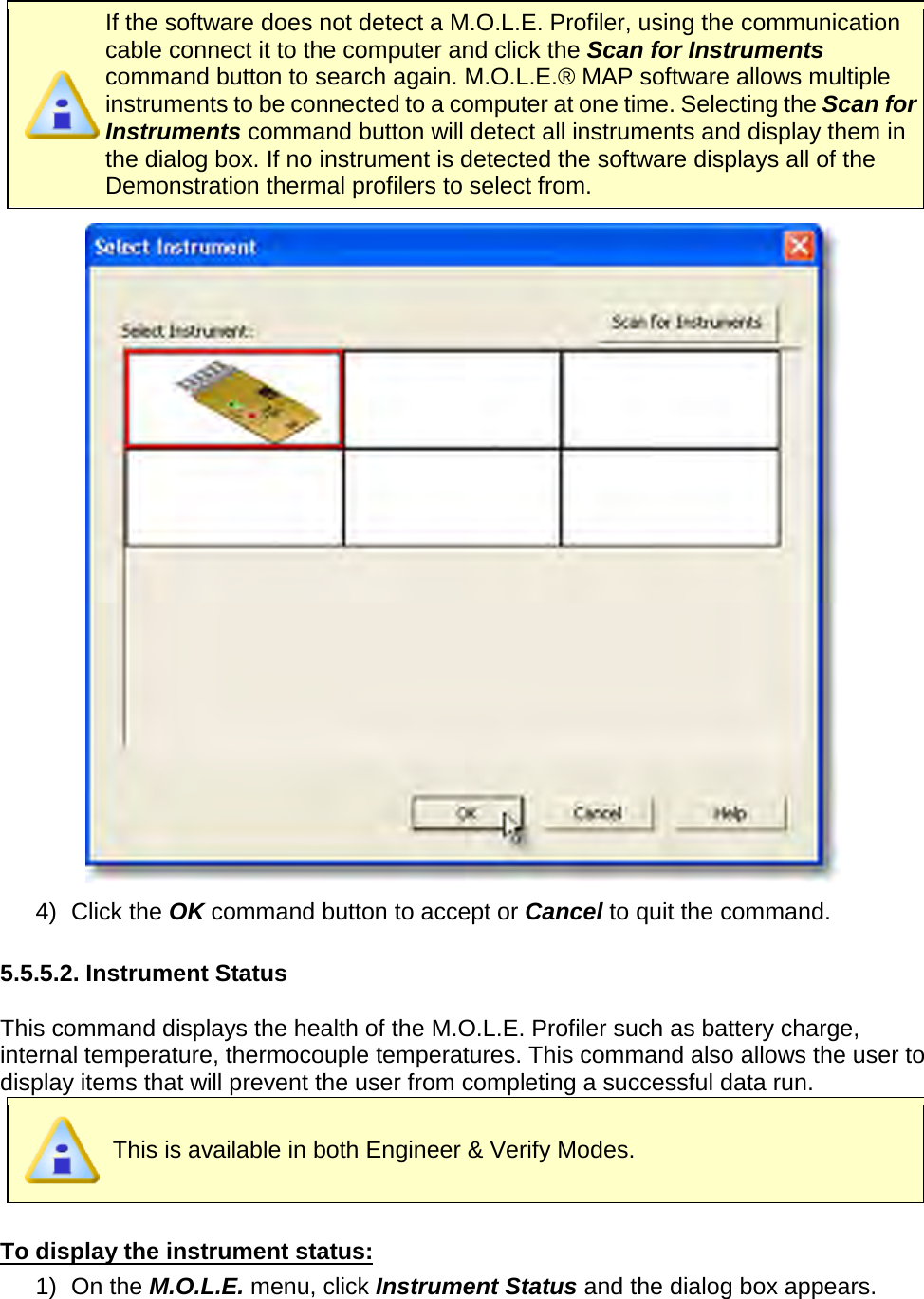
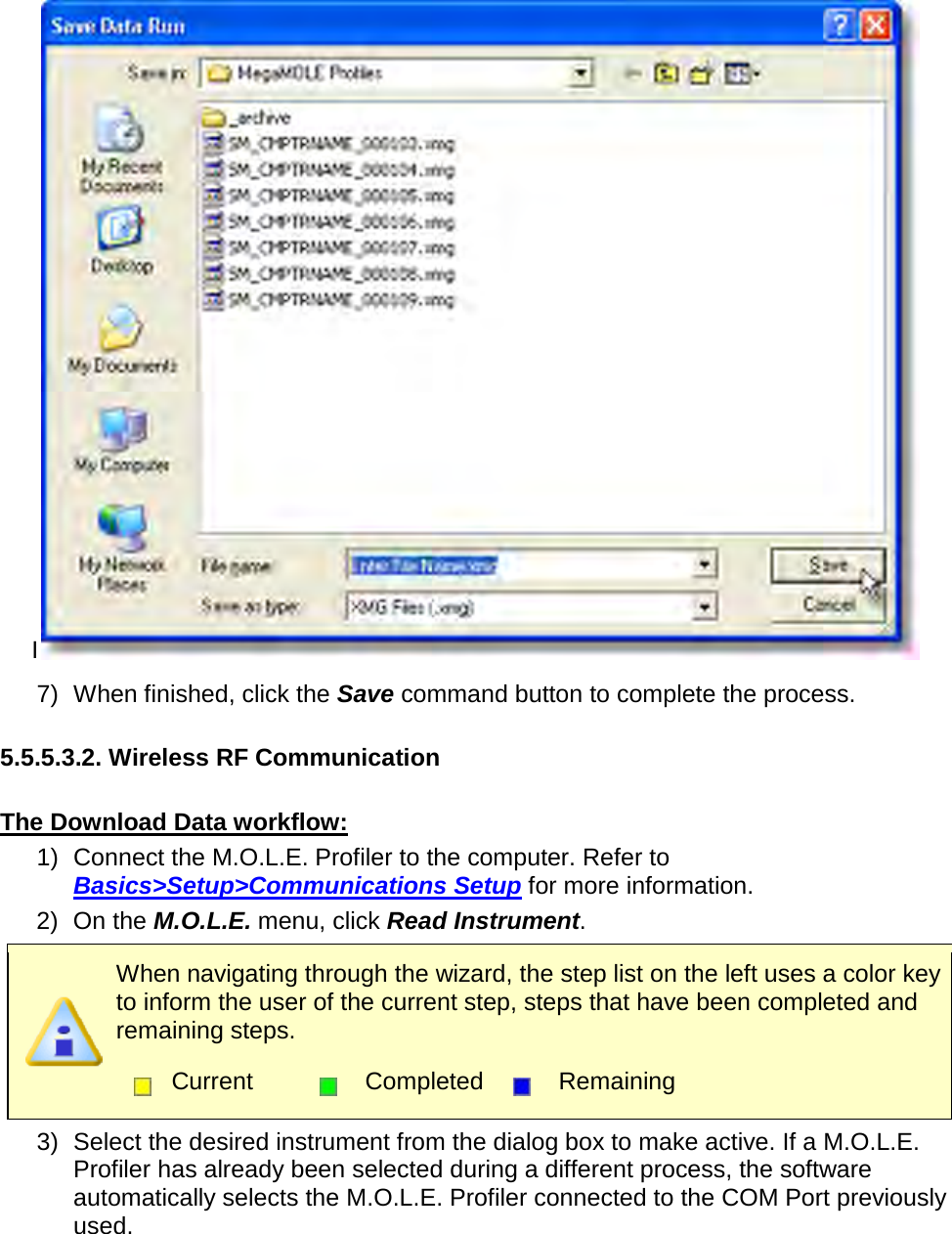
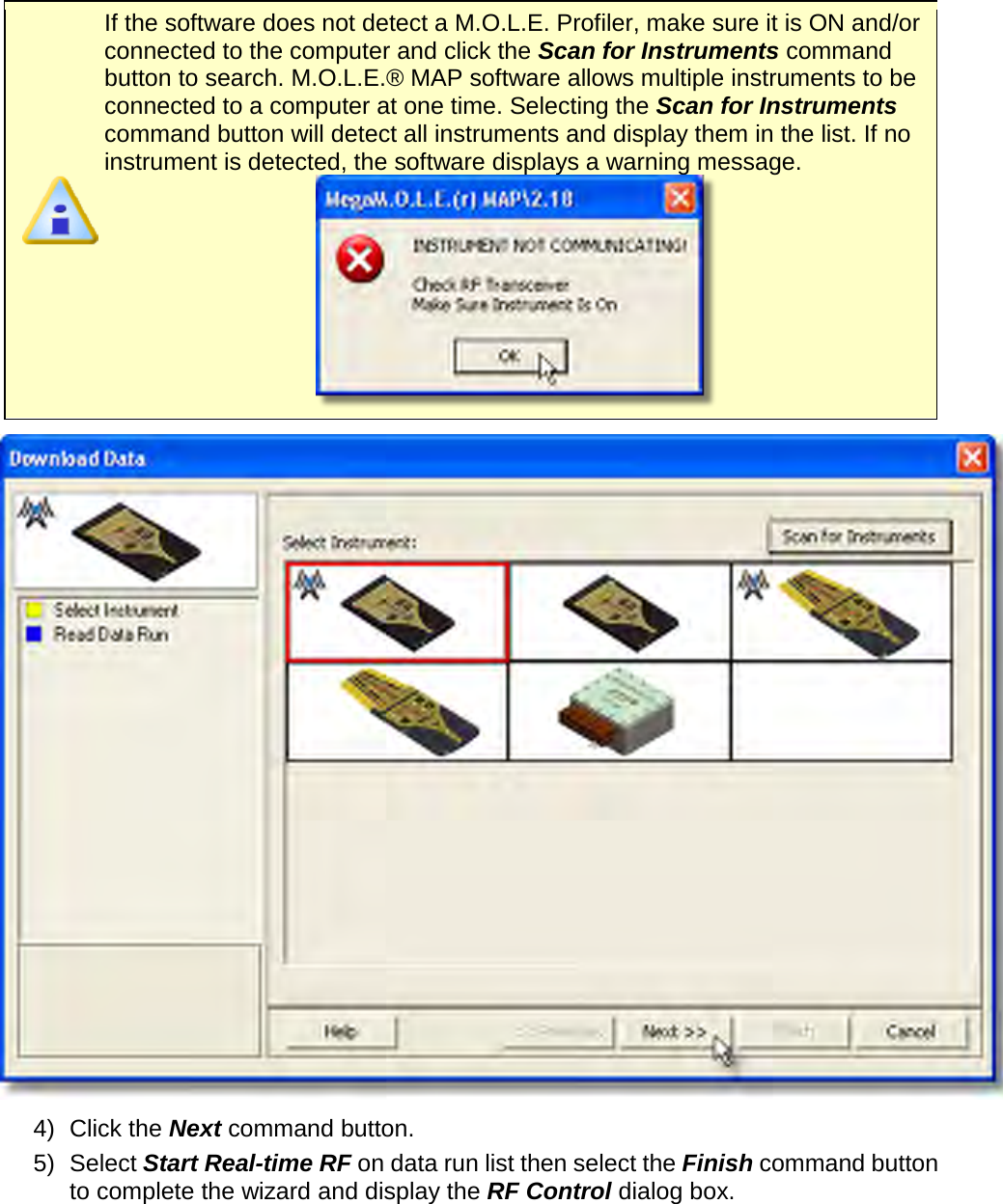
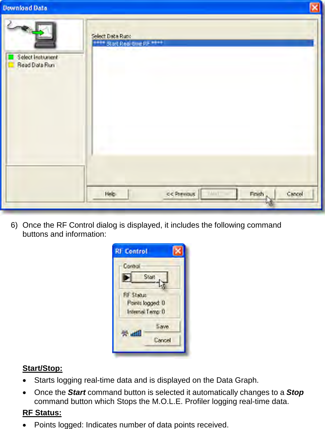
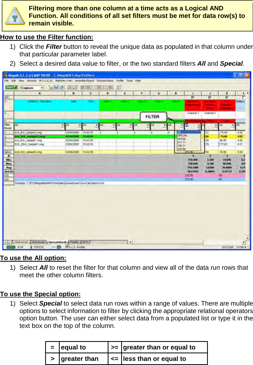
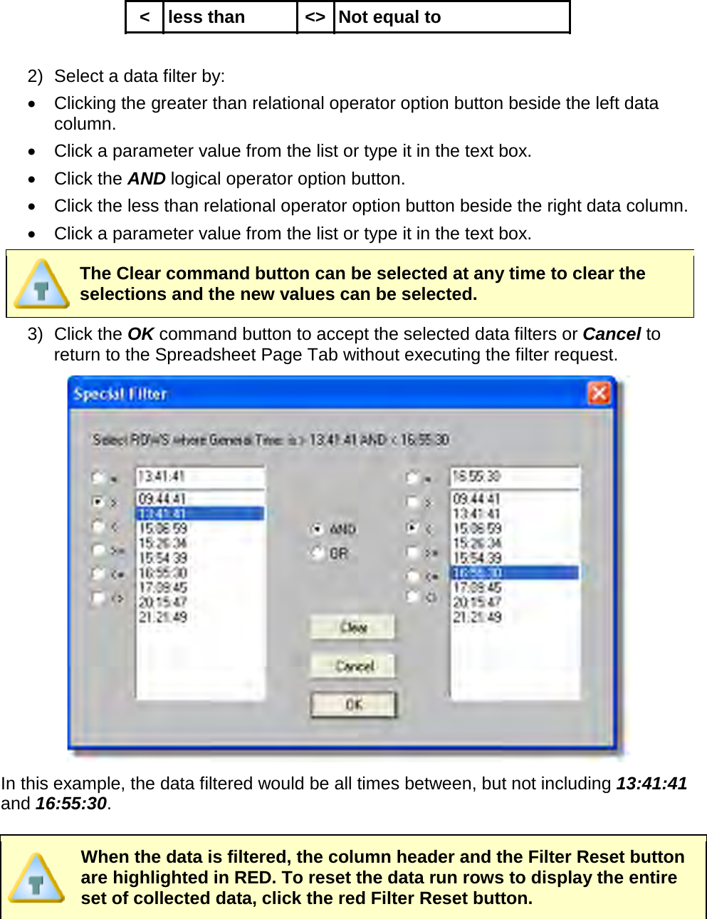
![5.4.3.5. Data Run Rows All of the data runs in the open working directory are listed on the Spreadsheet Page Tab as individual rows. The first data run uploaded or imported into the directory is on the bottom and the most recent data run is on the top. When any data run row is selected, all of the cells in the entire row are highlighted in purple and blue. The purple cells indicate that the cells can be modified and the blue cells indicate the data cannot be modified. When any individual data cell in a data run row is selected, all of the cells in the entire row are highlighted in green and yellow. The green cells indicate that the cells can be modified and the yellow cells indicate the data cannot be modified. When a data run row is selected, the data for that row will also be displayed in the Sel= row located at the bottom of the data run rows. This row allows the user to easily compare the selected data row to the statistics calculations located below the selected run row. Selected rows and columns can be “copied” by pressing keys [CTRL + C] and then “pasted” [Ctrl + V] into other applications. The data run rows can also be moved into any order desired. This is useful when the user wants to place similar data runs together. To change the order of the data run: 1) Select the number cell of a data run row with the mouse pointer. The row will then become highlighted in purple and blue. 2) Drag the row and drop it to a desired location. 5.4.3.6. Filters There are Filters for each parameter label that user can filter specific data out.](https://usermanual.wiki/Electronic-Controls-Design/E51-0386-40.User-Manual-part-2-of-3/User-Guide-1481866-Page-12.png)


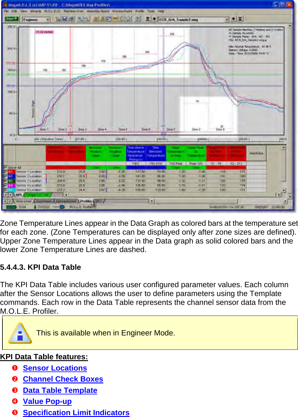
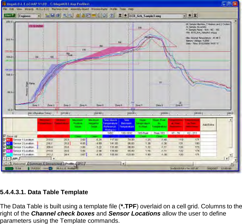
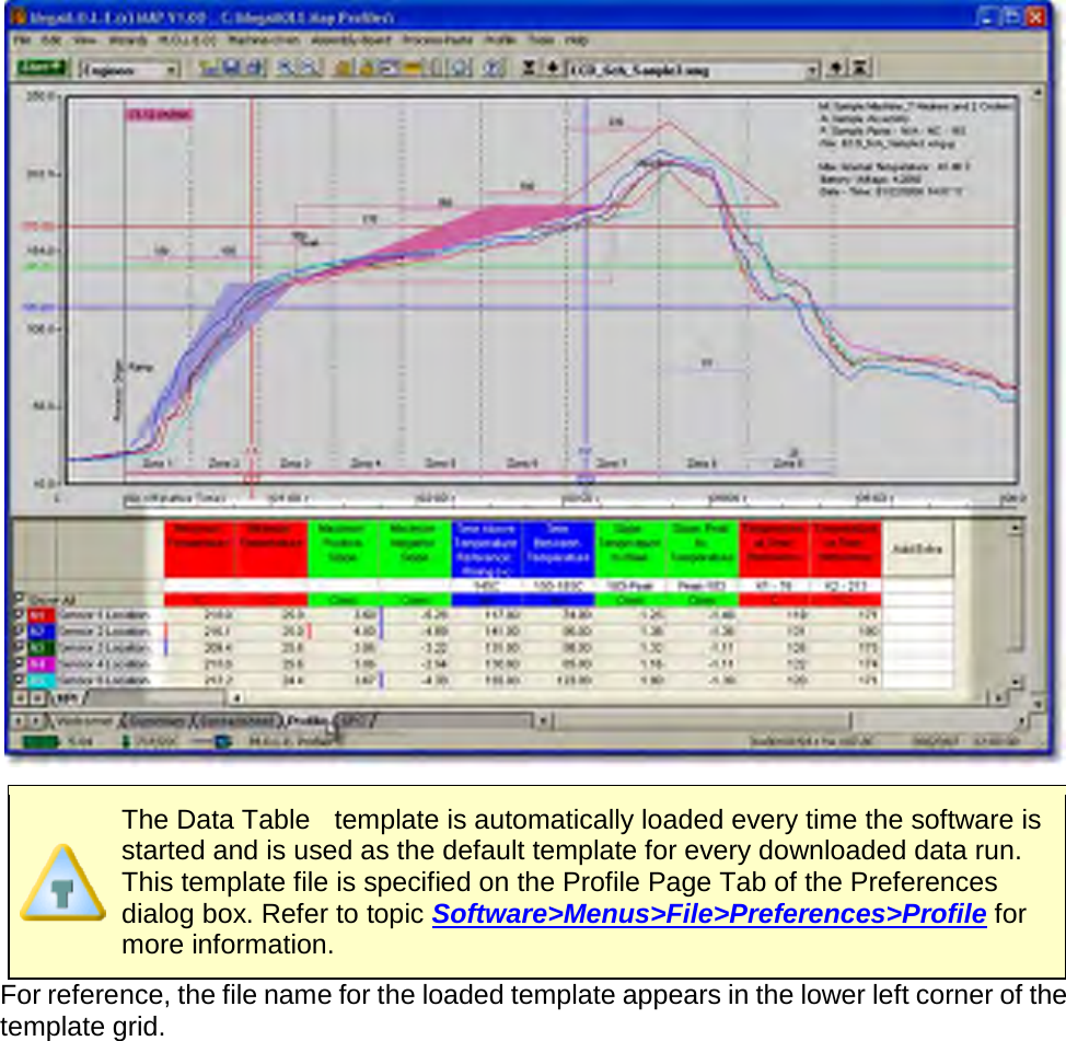


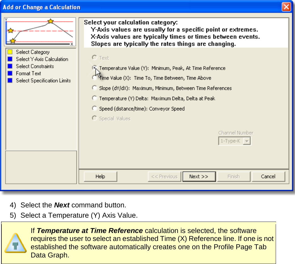
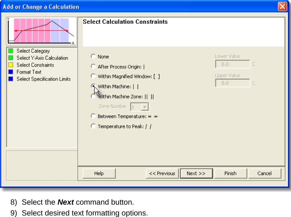
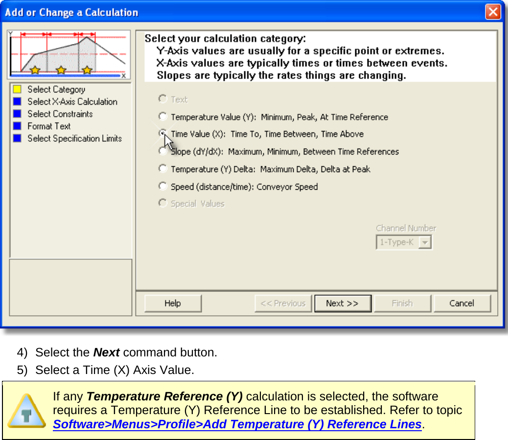


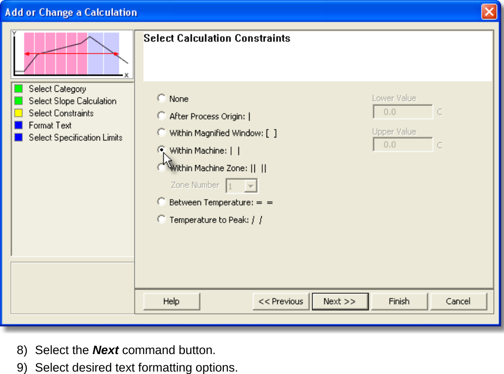


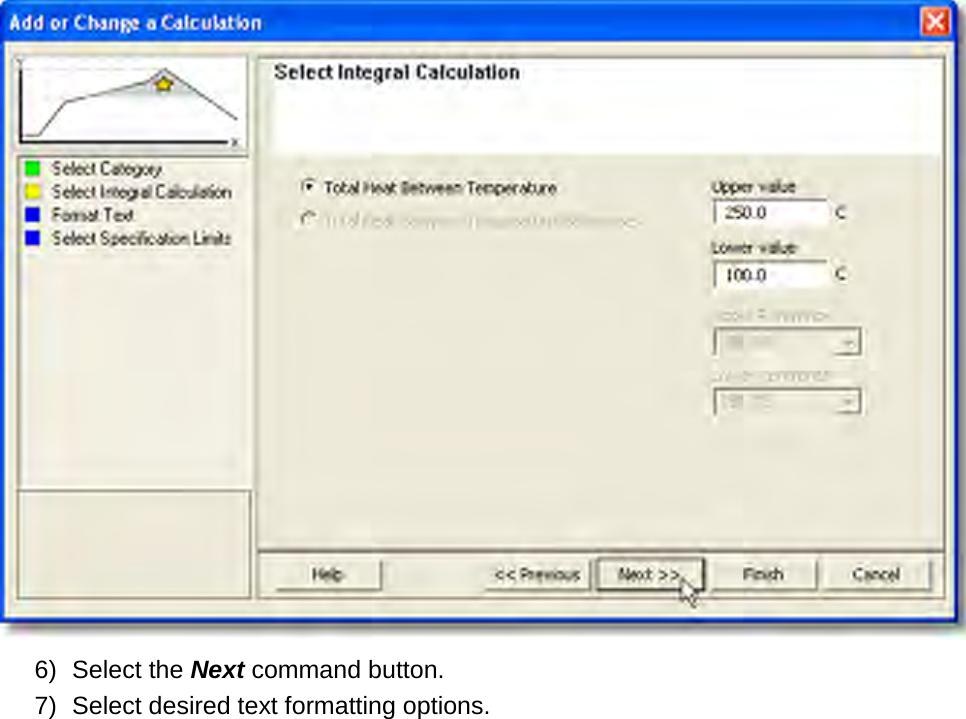
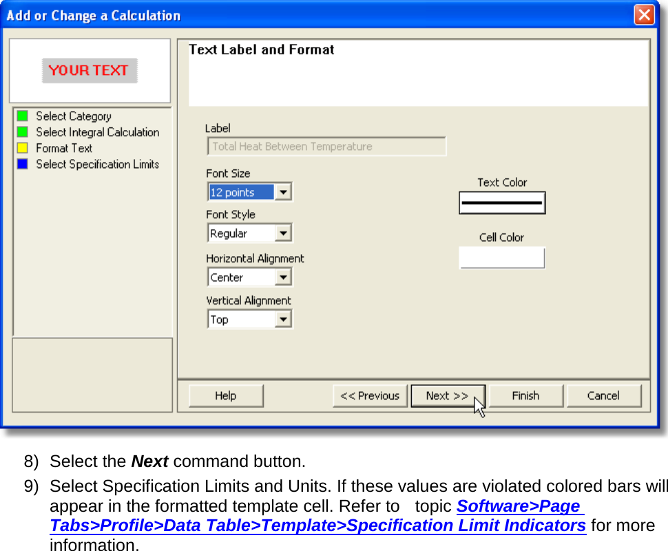

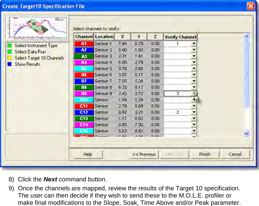
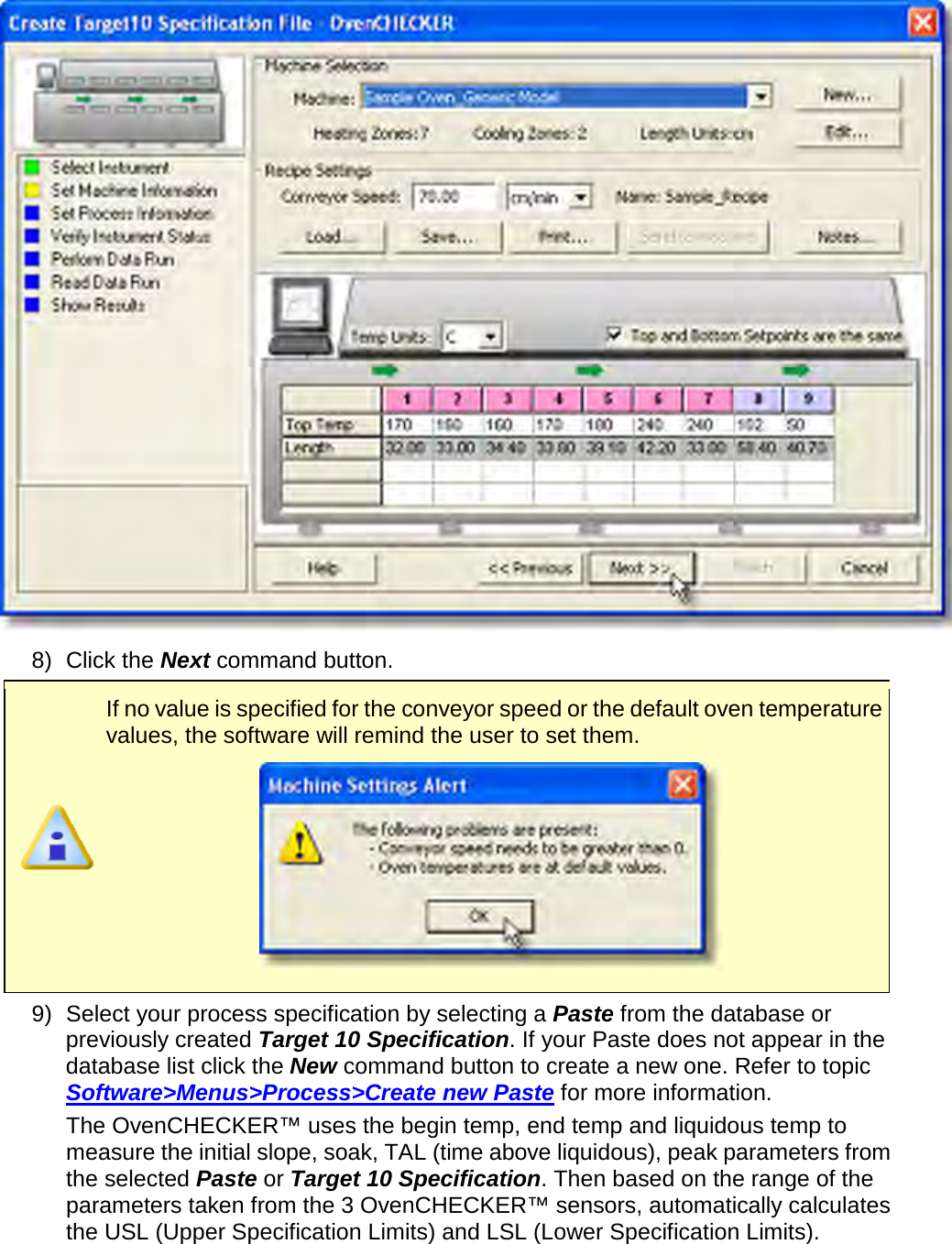
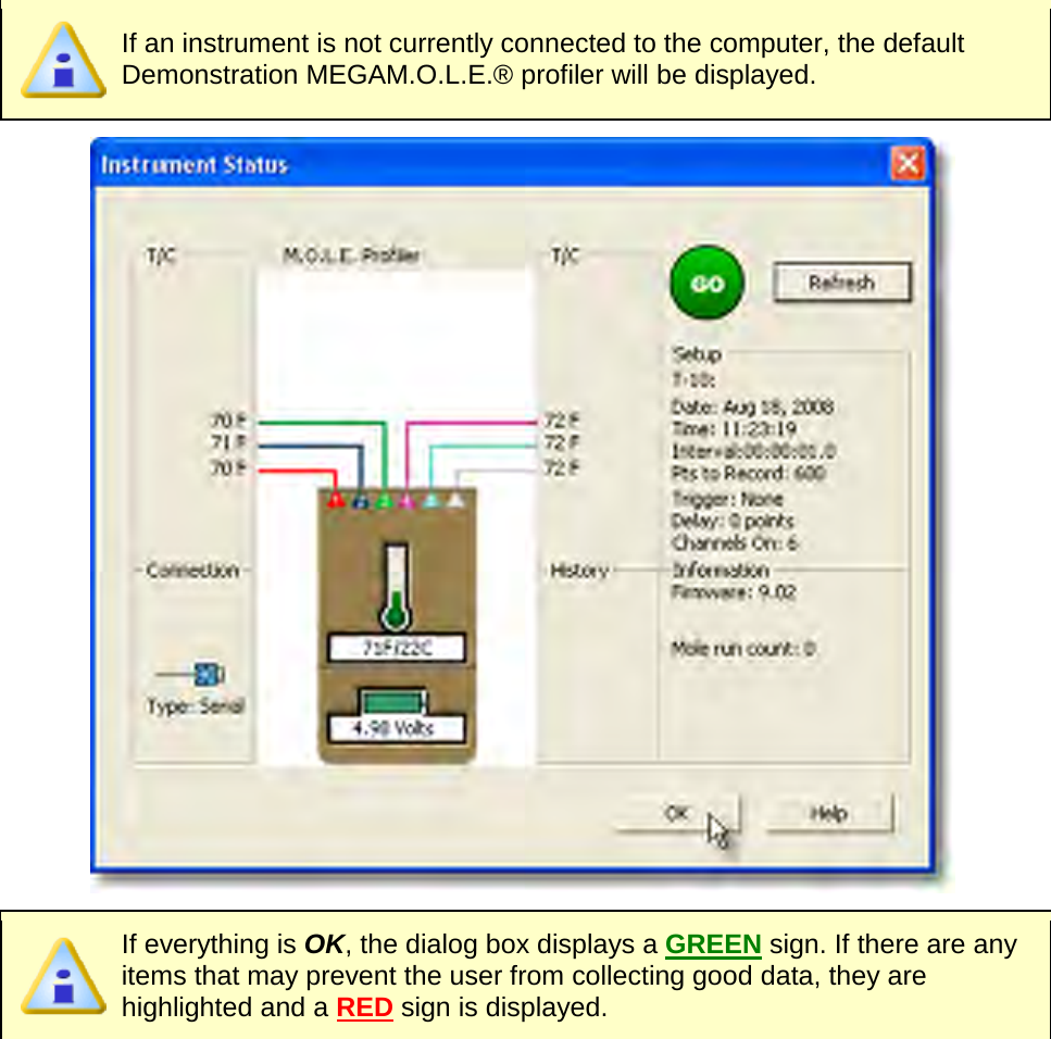
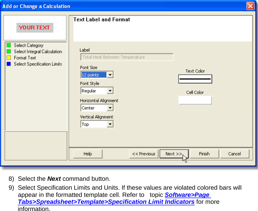
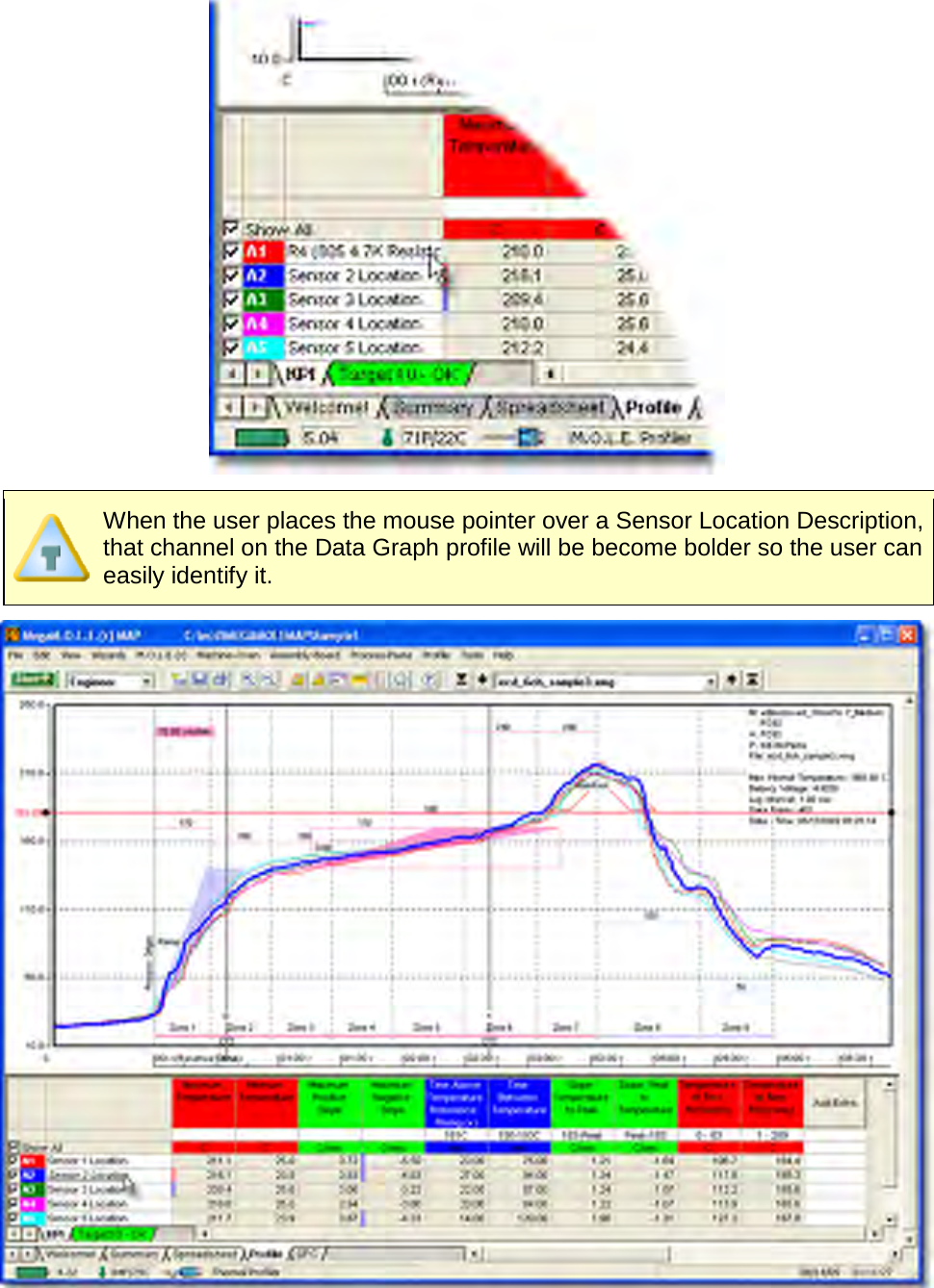
![Refer to topic Software>Page Tabs>Profile>Data Table>Template>Add & Edit Content Wizard for information on how to apply LSL and USL values. 5.4.4.3.2. Sensor Location Description The user can use the Sensor Location cells in the Data Table to describe the location where each sensor is connected to the test product. The color and description indicates which Data Plot on the Data Graph it represents. To change a Sensor location description: 1) Click a Sensor Location cell and type the desired name and press the [enter] key. The Sensor Location description can also be accessed by using the Set Assembly Information command in the Assembly menu.](https://usermanual.wiki/Electronic-Controls-Design/E51-0386-40.User-Manual-part-2-of-3/User-Guide-1481866-Page-67.png)
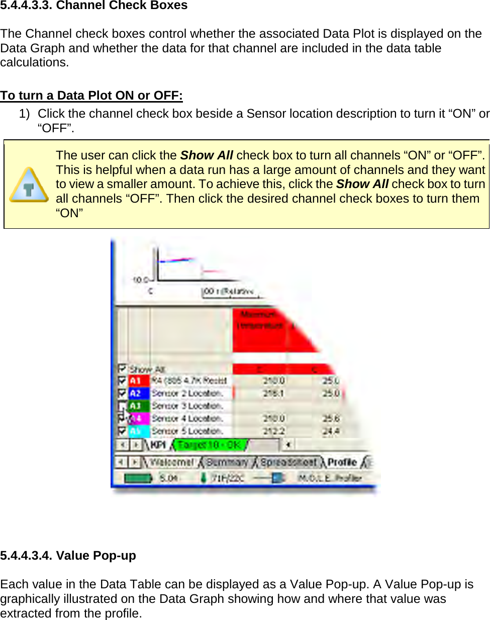
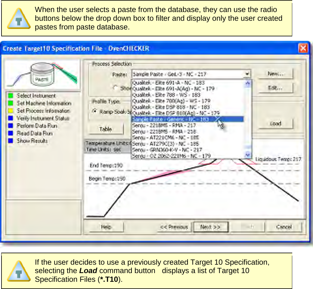
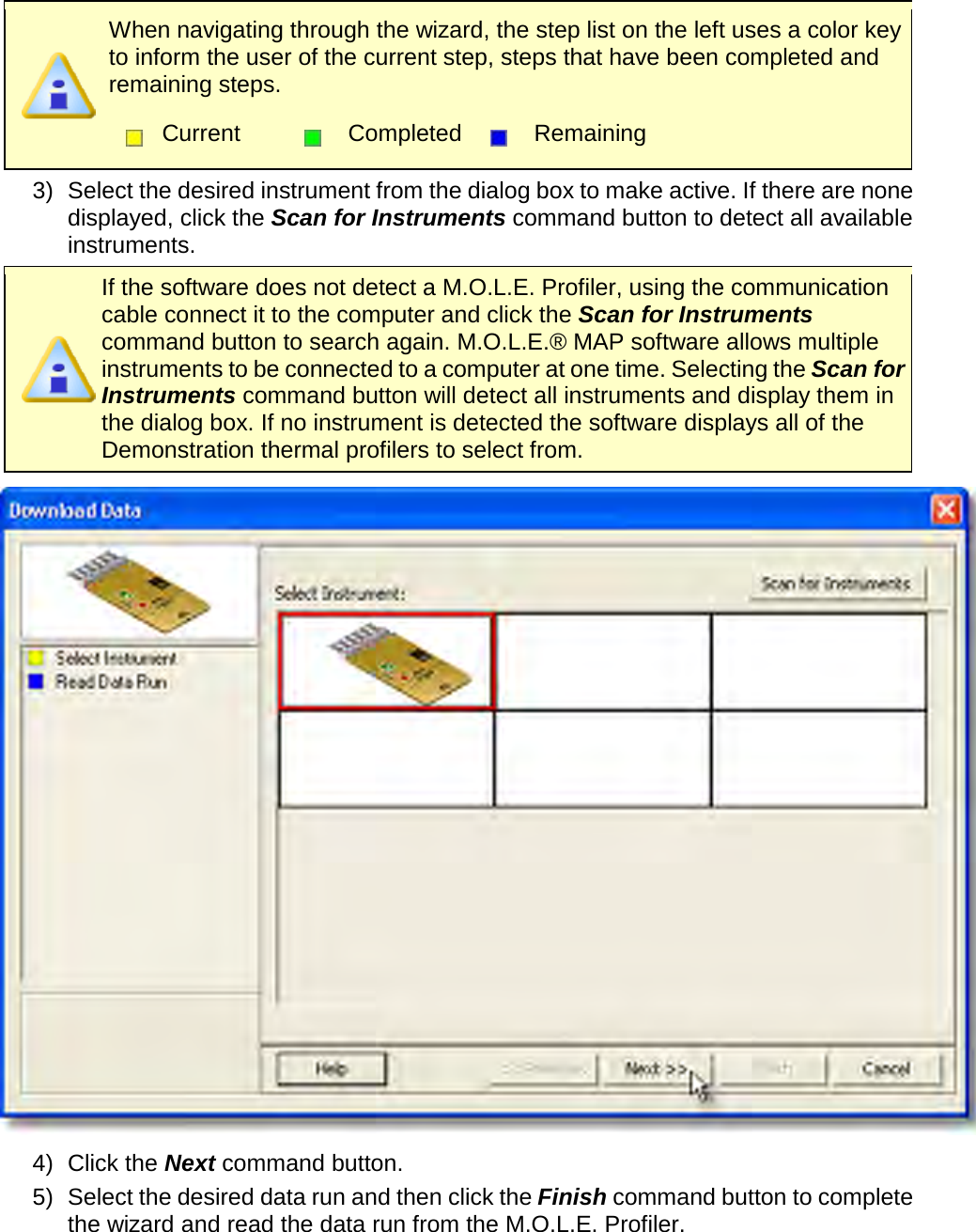
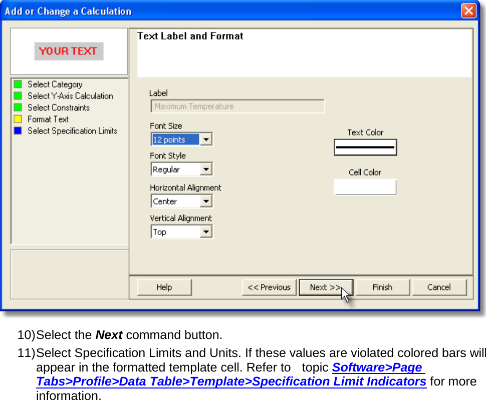
![To display a Value Pop-up: 1) Select the Profile Page Tab view. 2) Move the mouse pointer and hover over a desired value cell in the Data Table. That value will be displayed on the Data Graph where that value was extracted. To display more than one value pop-up at one time, left-click on each desired value cell. To print Value Pop-ups displayed on the Data Graph, they must be displayed using selection method. Value Pop-ups displayed using the hover method will not print. To remove a Value Pop-up: 1) Using the mouse pointer, select the object on the Data Graph by clicking it once. The object trackers will then become bold indicating that it has been selected. 2) Press the [Delete] key on the keyboard to remove the object. Additional methods to remove value pop-ups are, left-click on each value cell displayed or press the [ESC] key to remove them all at one time. Also, selecting a different page tab refreshes the Data Graph.](https://usermanual.wiki/Electronic-Controls-Design/E51-0386-40.User-Manual-part-2-of-3/User-Guide-1481866-Page-70.png)


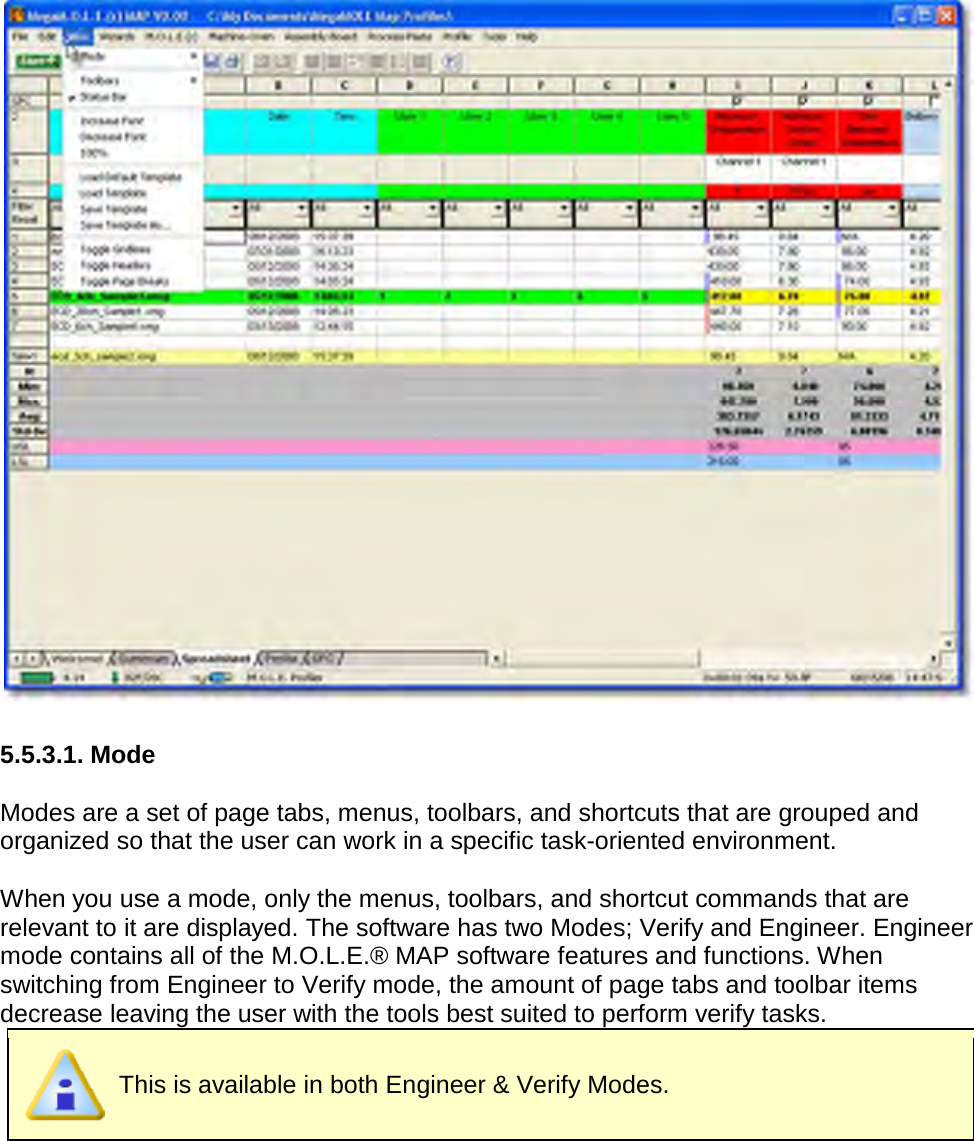
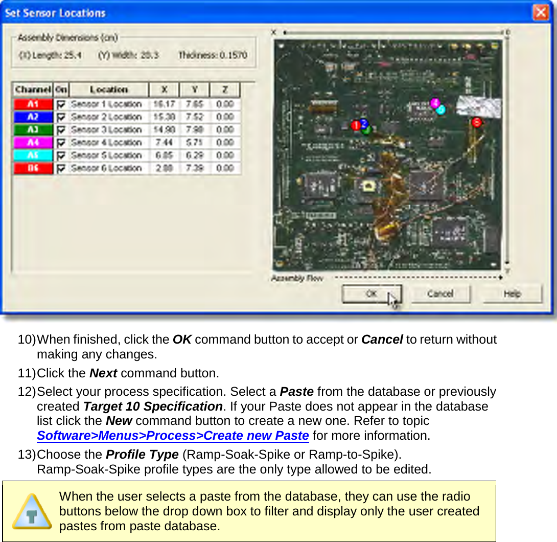
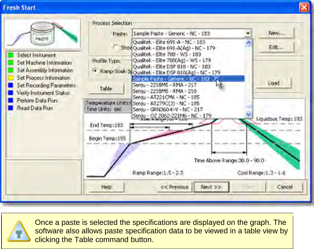
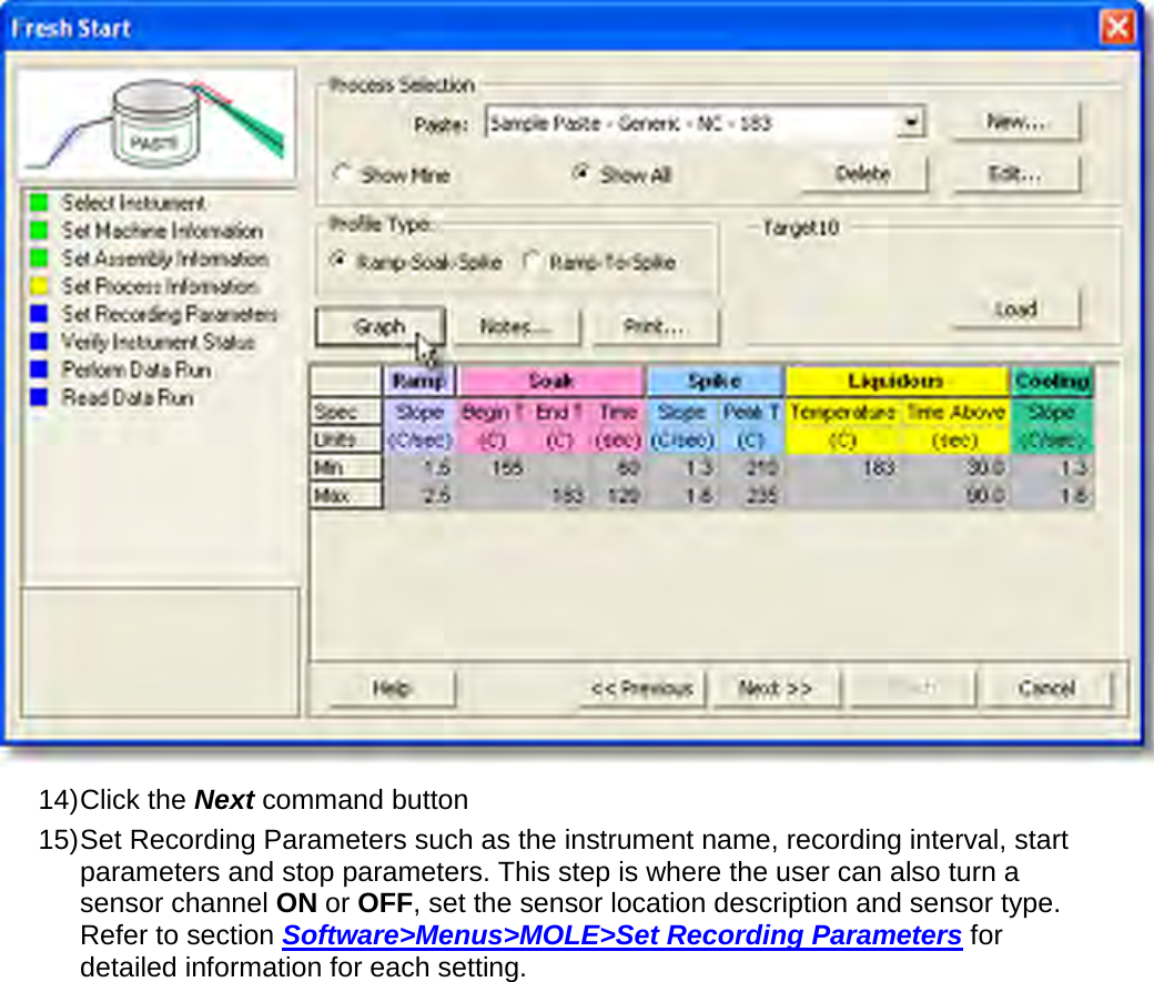
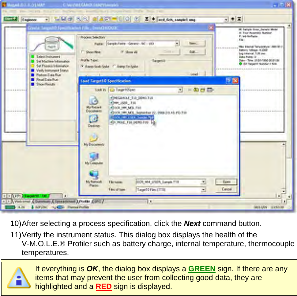
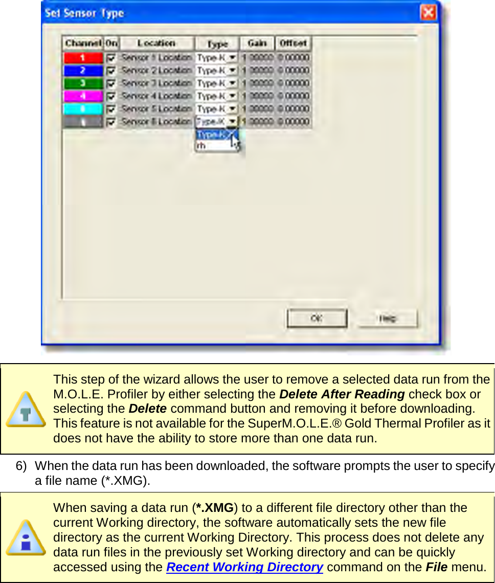
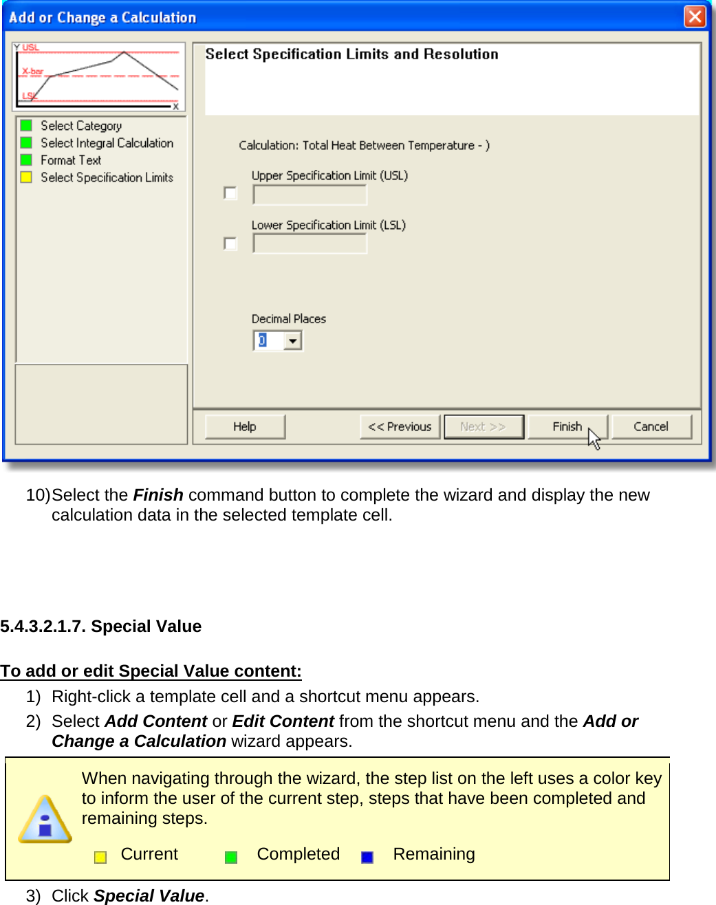
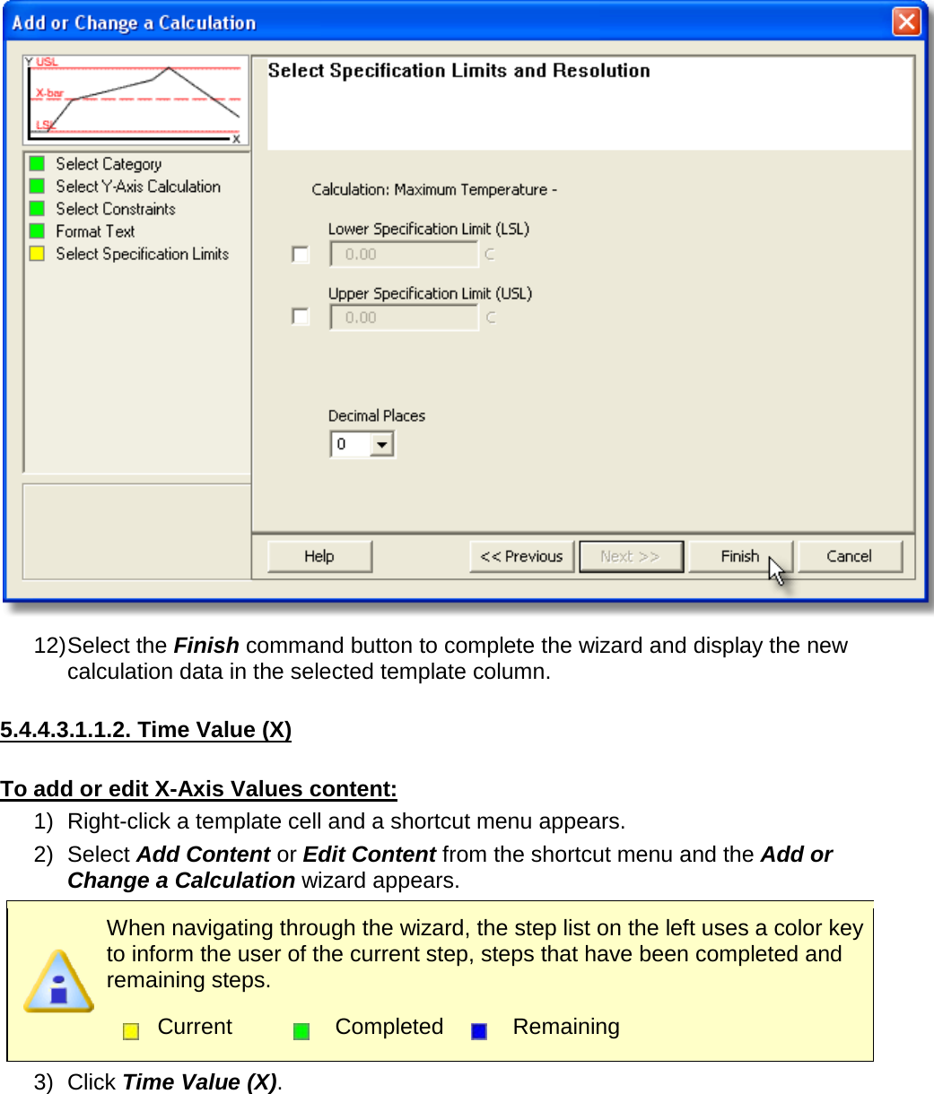
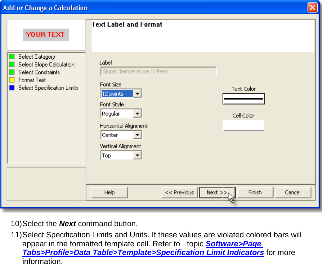
![5.5.2. Edit Menu The Edit menu commands enable the user manage the data run set displayed on the Spreadsheet to so the most beneficial data is assembled in the working directory. This is available in both Engineer & Verify Modes. 5.5.2.1. Copy To copy data: 1) Select the Spreadsheet Page Tab. 2) Highlight a Spreadsheet data run row or individual cell. 3) On the Edit menu, click Copy to copy the data in the selected Spreadsheet cells for pasting into other user definable cells or different programs. This command can also be used by pressing the shortcut keys [CTRL +C]. 5.5.2.2. Paste To paste data:](https://usermanual.wiki/Electronic-Controls-Design/E51-0386-40.User-Manual-part-2-of-3/User-Guide-1481866-Page-116.png)
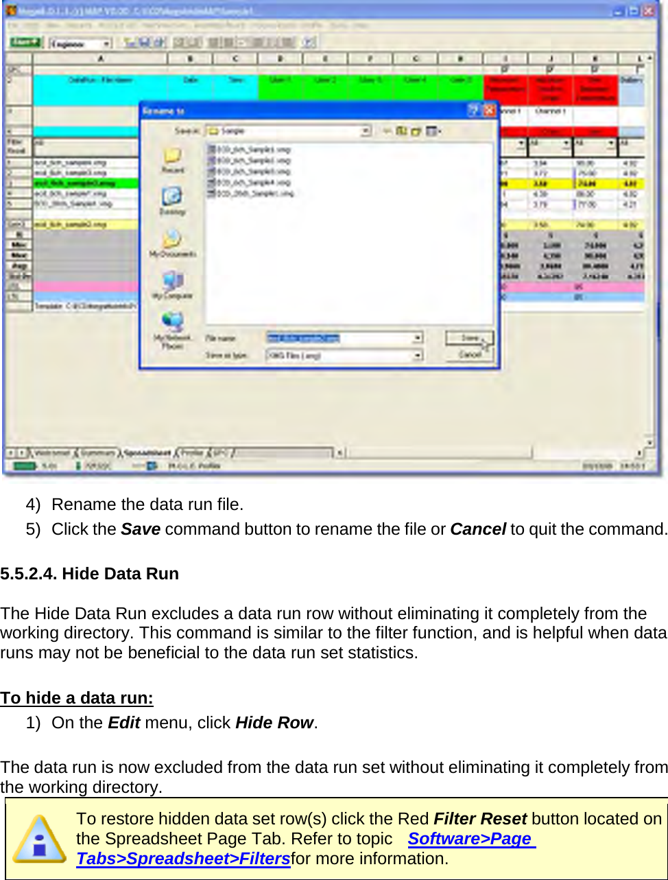
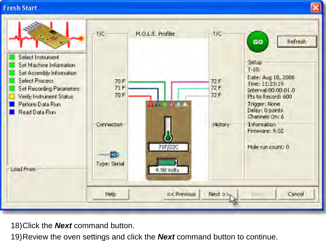
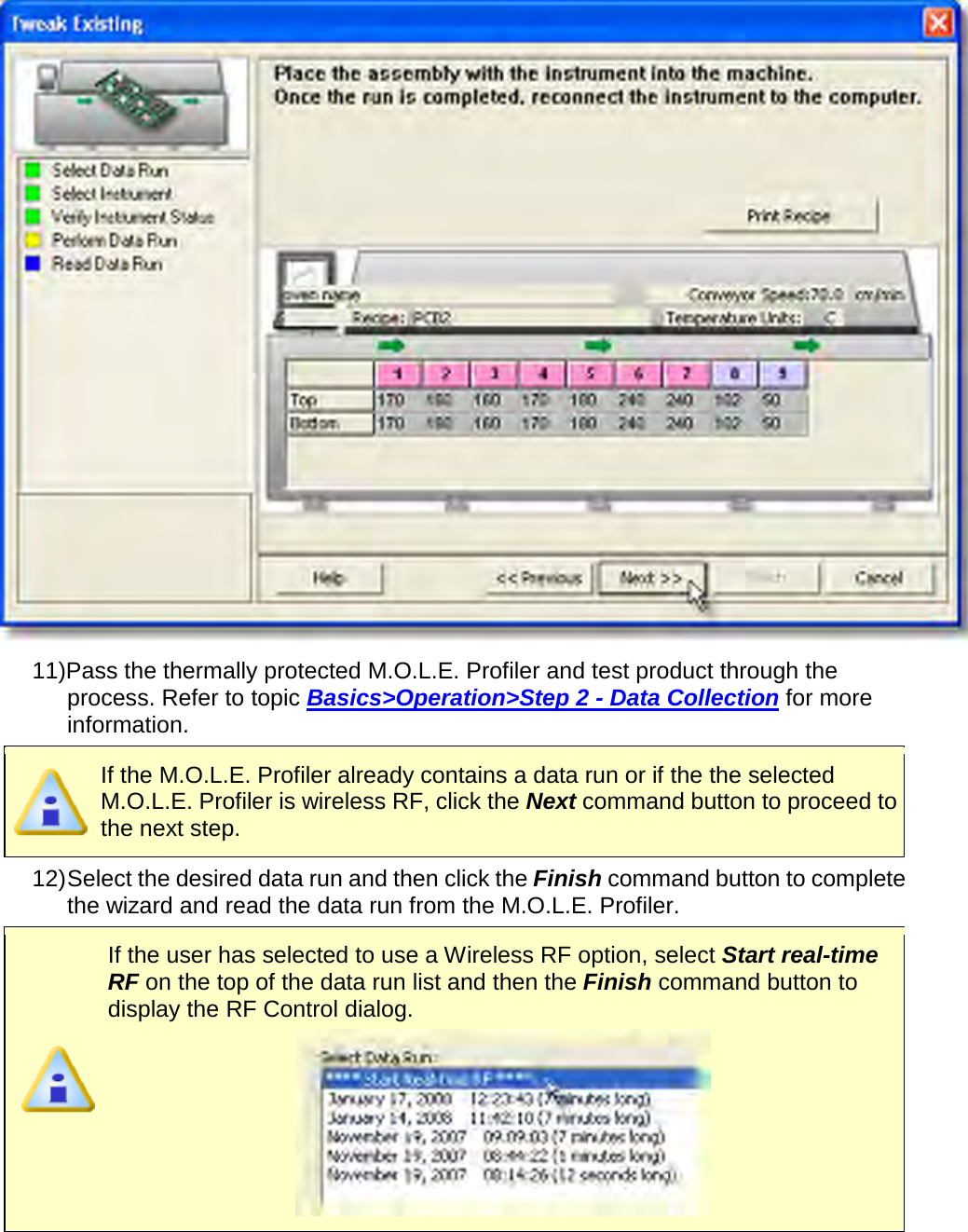
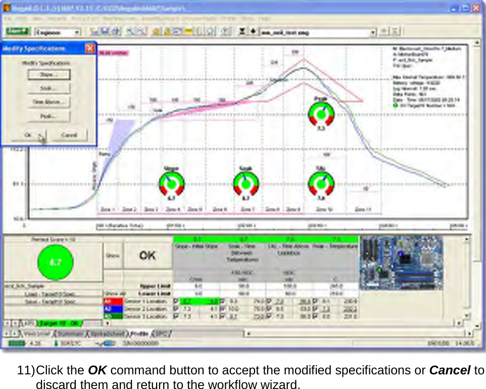
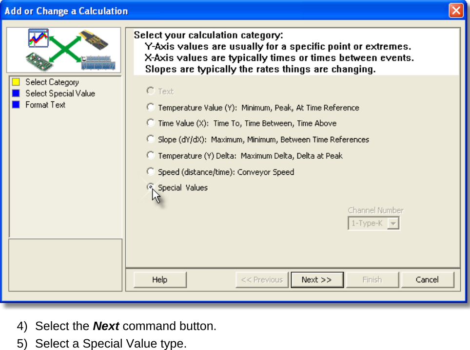
![1) Select the Spreadsheet Page Tab. 2) Highlight a user definable cell. User definable cells have label headers of User 1-5 and are colored green. 3) On the Edit menu, click Paste, to paste the data in the selected Spreadsheet cells. This command can also be used by pressing the shortcut keys [CTRL +V]. 5.5.2.3. Rename Data Run Since the software is a data run manager, the user can rename the data run files displayed on the Spreadsheet Page Tab. To rename a data run: 1) Select the Spreadsheet Page Tab. 2) Highlight a Spreadsheet data run. 3) On the Edit menu, click Rename Data Run and the software prompts the user to specify a new data run file name.](https://usermanual.wiki/Electronic-Controls-Design/E51-0386-40.User-Manual-part-2-of-3/User-Guide-1481866-Page-117.png)